

On the determination of Profit
On the determination of Profit
Updating my Rate of Profit Simulation and responding to CasP theory

This blog exists to accomplish two things, to provide an update to my simple rate of profit simulation, one of the first posts on my substack, and also to respond to the recent counter-critique by Capital as Power theorists that relates to my previous post. Both of these things relate to the importance of fixed capital investment and depreciation in determining profit.
Updating the Rate of Profit Simulation
The code for this simulation can be found here.
First, it is necessary to recap the logic and math of the rate of profit simulation in order to explain what needed to be corrected.
The simulation starts with 100 units of value, split into arbitrary proportions into the three main components of national accounts: variable capital (wages), constant capital (depreciation or capital consumption), and surplus (profit). From the initial arbitrary value of constant capital (C) the size of the initial capital stock is calculated, with the first ten years of the depreciation schedule equal to that initial constant capital value. The total value in the simulation will remain fixed at 100 and will represent the total labor budget of an economy at any given year, such that each variable will be automatically expressed as a percent of total income.
The simulation then proceeds to iterate through the following steps 100 times to produce the next proportions for V, C and S:
(note that substack doesn't let you use subscripts, so instead I'm using italics)
Because the capital stock is fixed in advance, the amount of constant capital is calculated first. This is determined by the fixed investment in the previous production cycles, or if this is the first one, by an arbitrary amount. The total amount invested is divided into 10 parts, assuming a ten year average depreciation schedule, which each form one year of the depreciation schedule. At the end of a production cycle, schedule years 1:9 are replaced by 2:10 and the 10th year is zeroed out.
C = cstock1 , where cstock2:10 represent Cn+1:n+11 in formation.
This represents a big improvement over my previous model, where depreciation was always to be taken as 10% of the capital stock, and therefore would not fully depreciate investment over a ten year period.
In the process of creating this model I decided to experiment with two different depreciation schemes. The first is the normal one, where the 10 depreciation schedule years each have equal amounts of depreciated value in them. The second is double declining balance depreciation (DDBD).
DDBD is an accelerated depreciation method where each year double the usual percent of depreciation is taken from the remaining balance. You can click the link for more details about how it works. In the simulation I wrote a function which operationalizes the logic.
Surplus is determined by subtracting C from total value, and then multiplying the remainder by the rate of exploitation(exp).
(Total - C)*exp=S, where exp is between 0 and 1
In this simulation, exp as a variable is defined exogenously, but the real life version is exp = S/(V+S), which contrasts to Marx’s original rate of exploitation formula of S/V. This change was done to make the math of the simulation work easier, expressing exploitation as a share of total living labor available, rather than as a ratio with income to capital.
Variable capital is determined in the same way, except with the value of the rate of exploitation inverted.
(Total - C)*(1-exp)=V, where exp is between 0 and 1
Capitalist consumption, the amount of resources capitalists use to reproduce themselves as a class, is determined next.
Here, and with the determination of investment, is where I realized I made a mistake in my previous simulation. Originally, this was determined by multiplying Surplus (S) by a rate of capitalist consumption (capconratio), where surplus was the same S as defined previously. However, I realized this was incorrect. In the Kalecki profit equations, which is where I got the idea that investment came from profit, depreciation is counted as a part of profit. Originally I dismissed this as unimportant and included depreciation as a cost like it is on firms income statements, until I realized that this is important to counting gross investment as a part of profit. This is because doing otherwise removes the role that depreciation plays in reproducing capital. Depreciation, by being counted as a cost, is essentially accounting for a certain amount of the value created. When wages are counted as a cost they are also an income on the other side of the transaction. But when depreciation is counted as a cost, it only decreases the capital stock. The revenue which is accounted for by the cost of depreciation is essentially earmarked for maintaining the capital stock at a given level, but this money doesn’t actually have to be used for investment at all, it could be consumed instead, like profit can be. Hence its place in the Kalecki profit equations. I adjusted the simulation accordingly.
(S+C)*capconratio = Capitalist Consumption, where capconratio is between 0 and 1
Like exp, capconratio is an exogenous variable that we get to decide outside of the simulation. In the real world, the Ratio of Capitalist Consumption is:
1-(Gross Investment/(S+C))
Compare this to the original S*capconratio = Capitalist Consumption
The same system is used to determine the amount of investment, but with the capitalist consumption ratio inverted.
(S+C)*(1-capconratio) = Capitalist Consumption, where capconratio is between 0 and 1
The profit rate for a given iteration can be calculated very simply as:
S/(C+V)
This basic simulation allows us to plug in values for either the rate of exploitation or the rate of capitalist consumption in order to see how the rate of profit changes over time.
Limits of the Model
Because investment decisions only affect depreciation in the future, and also because depreciation isn’t always fixed rate, we shouldn’t expect to be able to plug in the capitalist consumption rate and rate of exploitation for a given year and get the exact rate of profit of that year. Instead, simulating how the capital stock changes over time was meant to show what drives changes in the rate of profit in general. In this respect, however, by assuming a fixed depreciation rate there will be some divergence from reality.
Another limit of the model is its relationship to market value depreciation. Market value depreciation is when the value of an asset, and therefore the amount of depreciation appearing on the balance sheet, is determined by the assets current market value rather than its original cost. Market value depreciation is useful because it more accurately catches the costs of replacing the capital in question, whereas historic cost also has its uses in being less easy to manipulate for financial reasons. The model technically assumes a kind of market value depreciation rather than historic cost, it assumes that the market value of the capital stock will change in proportion to changes in the size of the economy, for the simple reason that the model variables are meant to represent shares of the total income.
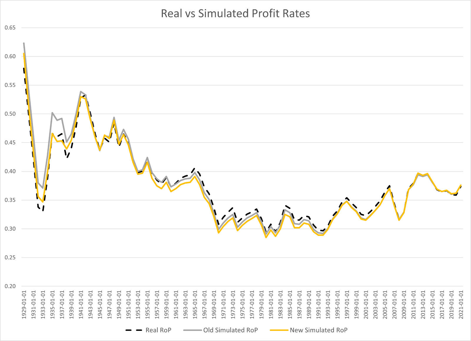
Comparing the Model to Real World Data
Plugging in the real world values for the rate of exploitation and the rate of capitalist consumption, we achieve a 99.3% replication of the real world profit rates, fairly impressive considering the limits of our assumptions related to depreciation.
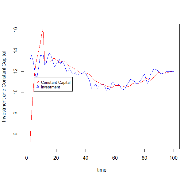
To see how much of an improvement this model is over the previous one, we can compare how either model approximated the rate of profit (r) and constant capital (c) .
As we can see, there is some real improvement of the approximation of constant capital, especially with the spike during the great depression much better approximated. The DDBD method in particular improved the correlation to real data the most at 80%, compare this to the 76% correlation of the normal depreciation method, and 74% of the method from the old model.

After my previous post there were some questions about why exactly the relationship between constant capital and surplus in my model wasn’t quite the same as the relationship in the empirical data. This graph hints at why. Since all the depreciation methods in the model overestimate the level between 1970-2010 somewhat, I believe the divergence isn’t the result of changes in the depreciation rate. Rather, it seems more likely that the market value of the underlying fixed assets did not grow as fast as the overall economy during this time.
To confirm this, I looked at the difference between nonfinancial assets at nonfinancial firms as counted in market values versus historic values, and turn this difference into a ratio of GDP. If we compare this to the differences between our simulation results and the empirical data, we can see there is a real relationship. Unfortunately, I couldn’t find equivalent data for fixed capital of private enterprises as a whole, which is the category relevant to the model, but this proxy does help to explain what’s going on even if it isn’t perfect.

Source on Market vs Historic Values/GDP
Moving on to the empirical rate of profit data, the improvements of approximating constant capital early on, particularly during the great depression, also created improvements in accurately simulating the rate of profit. From here on out, the depreciation used in these graphs will be the DDBD method since it is more accurate.
,
Updating Previous Findings on the Convergence of the Rates of Profit and Exploitation
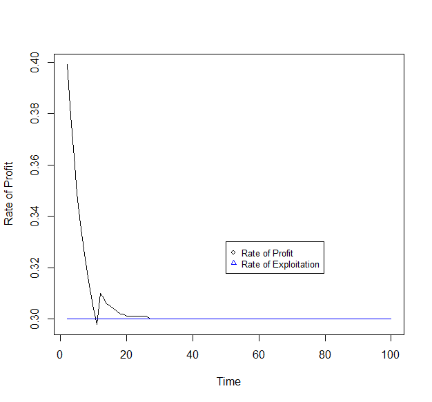
One important finding of the model that remains true in the updated version is that the ratio of investment and depreciation will always converge towards 1 over time.
However, another finding I stated in the old blog, that if the rate of capitalist consumption falls to zero that the rate of profit would converge to the rate of exploitation is in fact incorrect. With the model and corrected investment equations, the profit rate and exploitation rate will only converge if the rate of capitalist consumption is .5.
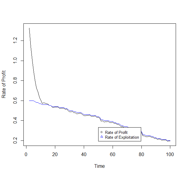
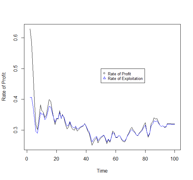
See the graphs below where the rate of capitalist consumption is .5, first when the rate of exploitation is fixed, then when the rate of exploitation is declining and then when the rate of exploitation varies according to real world data. The blue line represents the rate of exploitation.
.
.
This is because with the updated equations:
The rate of profit is S/(C+V), and the rate of capitalist consumption is Investment/(S+C).
Because investment always converges to depreciation, the rate of capitalist consumption can be rewritten so that it equals C/(S+C).
When capconratio is .5, that means ½=C/(S+C)
If C+S = 2C
Then C+S = C+C
S=C
Plugging that back into the rate of profit equation, we can substitute S for C. S/(S+V).
This is equivalent to the rate of exploitation which is S/(S+V)
This convergence can be observed empirically: as the ratio of investment to depreciation moves to 1 in the real world, so does the ratio of profit rates to the rate of exploitation.


Similarly, while our real world rate of capitalist consumption isn’t quite .5, it’s not too far off, falling between .55 and .66 since 1980.
Re-Cap of CasP Theory
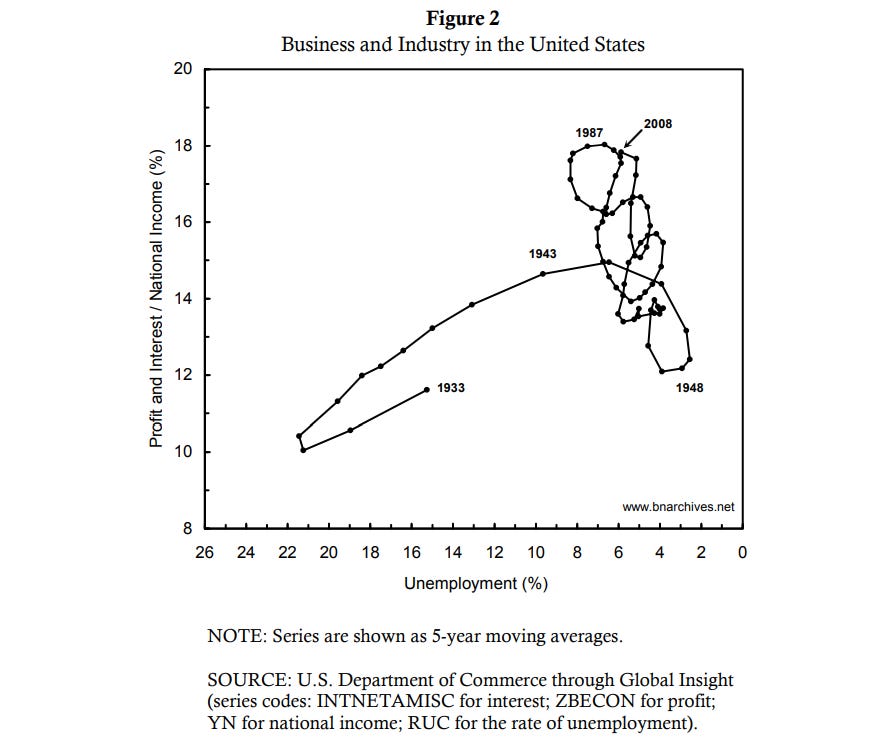
CasP theorists attempted to explain changes in the profit share of income with the unemployment rate, suggesting a parabolic relationship that led to lower profits at very low unemployment rates.

.
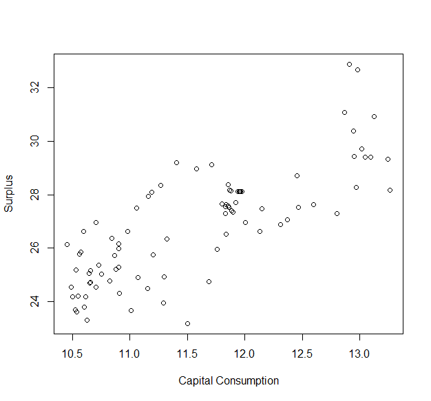
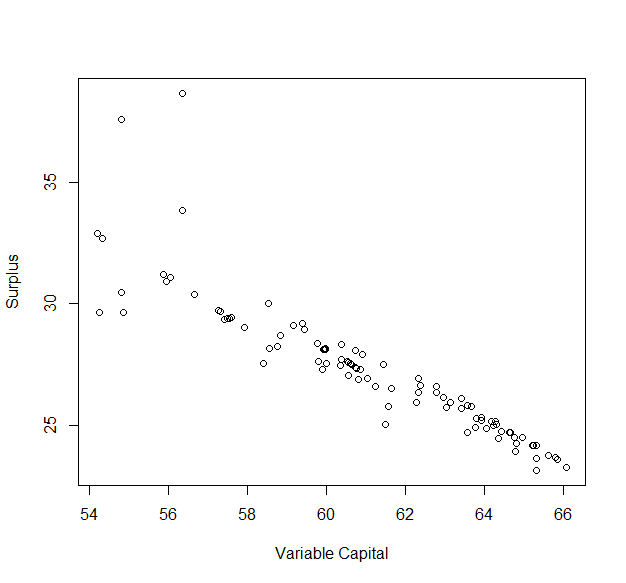
In my last post I disputed this evidence, including by constructing my own scatterplot of the relationship between capital consumption share of income, or constant capital, and profit share of income. For the purposes of this current post, I’ve also included a graph on the relationship between variable capital (employee compensation) share of income and the profit share of income.
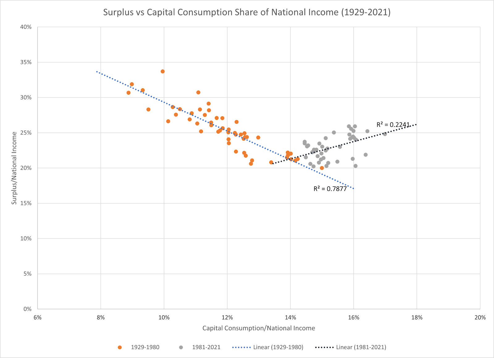

The relationship between capital consumption and profit experiences a change in dynamics after 1980, going from a strong negative relationship to a relatively weak positive relationship. In contrast, the relationship between employee compensation and profit has a straightforward negative relationship, though not as strong as that of the pre-1980 relationship of capital consumption and profits. I did also try dividing up the employee compensation share of income in terms of pre vs post 1980 data, however the strength of the relationship stayed about the same (an R of .52 and 56 respectively). Because I’ve split the data up by date, it’s important that I justify this so that it doesn’t seem that I’m simply trying to create a stronger relationship than there actually is, specifically by explaining how the dynamics which produce this correlation have changed after 1980.
Simulating The Systemic Shift in the 1980s
To do this, I can create this same kind of scatter plot in my simulation, and furthermore, by using real world data for for the rate of capitalist consumption and the rate of exploitation, I could decompose the real world effect of both on profit by plugging them into the simulation while holding the other variable constant at its real world average level. Once this is accomplished, we can look at the correlation between S and C on the one hand, and S and V on the other.
When we vary only the rate of capitalist consumption, we get correlations like this:

Like the pre-1980 data on capital consumption and profit shares of income, there is a negative correlation.
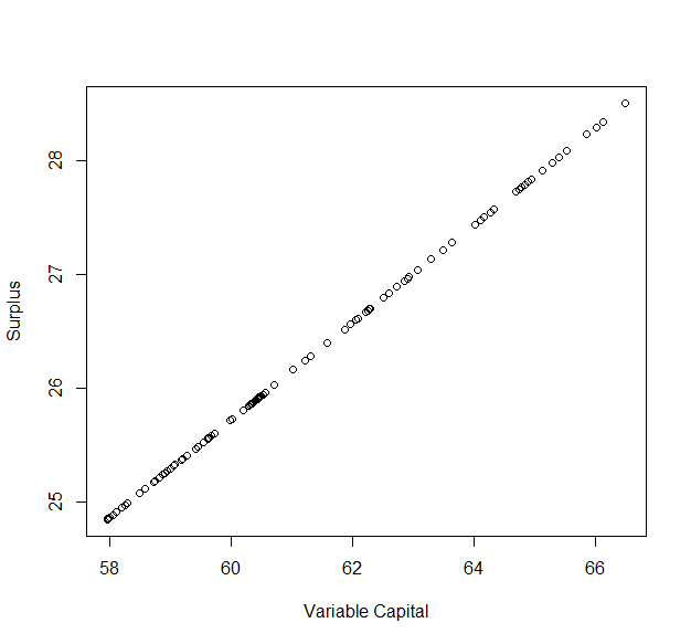
But unlike the empirical data, there’s a positive rather than negative correlation between Profit and Variable Capital, which here is equivalent to the employee compensation share of national income. This is because as constant capital increases and the rate of exploitation stays the same both Surplus and Variable capital will decrease at the same time and vice versa. Indeed, the relationship between the change in Constant Capital to Profit and Variable Capital can be expressed in the following equation when there is no change in the rate of exploitation:
(ΔC * -1) *exp = ΔS
(ΔC * -1) *(1-exp) = ΔV
These equations also imply that whatever the change in constant capital, the corresponding inverse change in Surplus and Variable Capital will be smaller, assuming exp does not equal zero or one.
When we run the simulation while varying the rate of exploitation and holding the rate of capitalist consumption fixed at its average, we get very different results.

More interesting is what happens when we exclude the first 15 points to see what tendency the simulation settles into.
In this case there is a mostly positive correlation between Capital Consumption and Surplus, this is due to the same effect we observed earlier but now in reverse, where the rate of exploitation increasing will increase the amount of surplus, and thus the amount of investment given a fixed rate of investment. The reason the correlation is weaker is due to the simple fact that while a change in Capital Consumption as a share of total value affects the amount of Surplus and Variable Capital that iteration, changes in the rate of exploitation can only affect the amount of investment which determines Capital Consumption and other proportions in the future.
As for the negatively correlated outliers at lower values of Capital Consumption, this is due to the simulation moving into equilibrium and Depreciation converging with Investment.
When it comes to Variable Capital things are much more straightforward. There is a negative correlation between the two, though not as clean as the relationship when the rate of capitalist consumption was being varied, as this time Variable Capital was being partly determined by investments made in the past, which is the other side of what we mentioned earlier.
Now, if we use both the real world data for the rate of exploitation and the rate of capitalist consumption, we can compare the simulated results to the real world results.
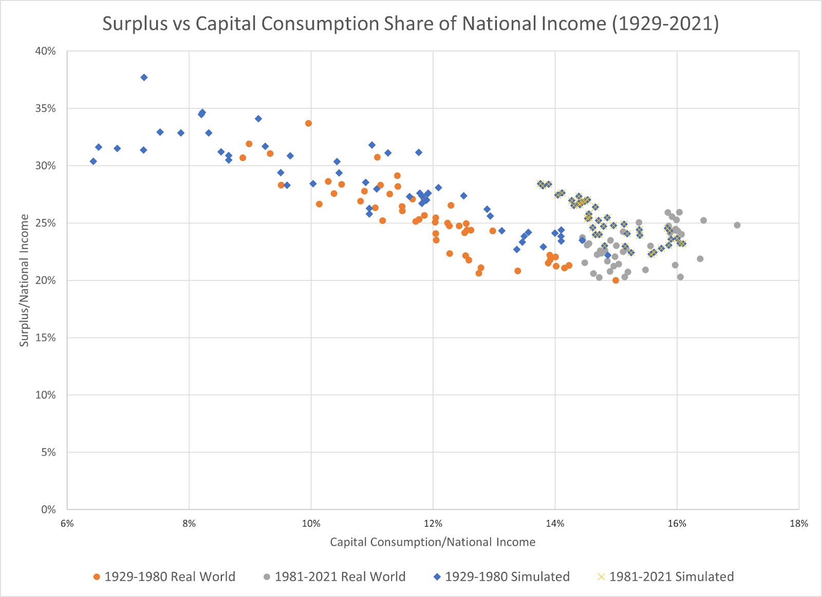
While the trend lines for each section are not quite identical due to the effects we discussed earlier about growth of market value diverging from economic growth, it’s clear that the simulation can approximate the real values fairly well. Both the simulation and the real world data confirm a fundamental regime change between pre-1980 and post-1980. As I’ve discussed previously, before 1980, the traditional Marxist idea of the tendency for the rate of profit to fall due to increasing fixed capital costs held, as surplus and capital consumption (aka depreciation aka constant capital) had a linearly negative relationship. This relationship began to breakdown afterwards due to the onset of neoliberalism.
I created this simulation, originally, to show how profit rates were determined. It allows us to decompose the causal effects of changes in investment/consumption decisions versus changes in how income is split between labor/capital. We can see these effects clearly by comparing the three different simulations with the real world rate of profit data.

Here, CCR refers to capitalist consumption ratio and EXP refers to the rate of exploitation. As one should expect, the simulation that used both sets of data is the closest to the real observations. We also see that the simulation that uses the rate of exploitation data appears more accurate than the one that only uses the capitalist consumption ratio, and this is true from a purely correlation sense. However, what the CCR simulation does very well is reveal the secular trend in the rate of profit, even if the EXP simulation is excellent at showing the cyclical changes in the rate of profit. For Marx, it was changes in investment, the capital stock and depreciation which totally determined the secular rate of profit, and were the force behind his theory of a falling tendency.
What has changed after 1980 is very simple, the secular trend in the rate of profit stalled and slightly reversed. We know from the various simulations that when secular changes are being driven by capitalist consumption/investment that the relationship between constant capital and surplus is negative. And we also know that when secular changes are being driven by changes in the split of income to capital and labor that the relationship between constant capital and surplus is positive. These two different paradigms describe very well the difference between the pre and post 1980 regimes. While the EXP simulation alone may appear closer to the real rate of profit visually, it doesn’t capture the reality of the pre 1980 relationship between constant capital and surplus.
Determining changes in surplus with respect to either constant capital or variable capital, using a causal model like this, is rather difficult unfortunately. This is because, unlike simply comparing the relative changes in each variable, the changes to S in the simulation are determined, and in some ways overdetermined, by the previous iterations and in a non-linear way. To understand the difficulty of formalizing this relationship, we must look at the central question I’ve been posing here, what determines changes in surplus.
Let’s return to the basic value equation.
Total Value = V + C + S
This means that any change in S/Total will necessarily entail a change in either C/Total or S/Total. Let me repeat this for emphasis: any change in profit share of income must necessarily, as a tautology of accounting, be reduced to a change in either a change in depreciation as a share of value, or wages as a share of value.
Accordingly, any change in S is equivalent to the negative changes in C and V:
∆S = -∆C -∆V
To see how the simulation changes this equation from a logical one to a causal one, we must expand it using the logic set out from the write up of the model.
∆C = Cn - Cn-1
Cn = (∑In-1:n-11/10)
Cn-1 = (∑In-2:n-12/10)
thus
∆C = (∑In-1:n-11/10) - (∑In-2:n-12/10)
where I = Investment and 10 is the length of the depreciation schedule. For the sake of simplicity I’m representing the normal depreciation method.
All this means is that constant capital is equivalent to 1/10th of the sum investment of the previous ten production cycles.
and
∆V = Vn - Vn-1
Vn = (100-(∑In-1:n-11/10))*(1-expn)
Vn-1 = (100-(∑In-1:n-11/10))*(1-expn)
thus
∆V = (100-(∑In-1:n-11/10))*(1-expn) - (100-(∑In-1:n-11/10))*(1-expn)
Therefore:
∆S = - ((∑In-1:n-11/10) - (∑In-2:n-12/10)) - ((100-(∑In-1:n-11/10))*(1-expn) - (100-(∑In-1:n-11/10))*(1-expn))
And this is not even including the equations which determine Investment, which is always a certain share of S, making it determined by that whole equation listed above and thus every previous iteration.
This makes it difficult to come to systematic conclusions besides saying that changes in Surplus ultimately come down to changes in investment and changes in the rate of exploitation.
Returning to the logical and empirical analysis of ∆S = -∆C -∆V , we can break down the extent to which historical changes in S were due to C and V. The limit of this kind of analysis, and the value of the simulation, is that the simulation can consider counterfactuals due to its causal and temporal basis. If we were to hold V constant in real life we wouldn’t expect C to go on exactly as it would with V varying normally, C would change in some way because V is not changing. The simulation can capture some of that change. On the other hand, the empirical data is more concrete and also illuminates something important that people such as the CasP theorists overlook.

From 1929 to 1980, surplus declined by -14.5 percent of total, while variable capital increased by 8.9% and constant capital increased by 5.6%. If we combine the negative change in V and C we get an amount equivalent to the negative change in S, which is to be expected. In this case, the rise in constant capital was the direct source of nearly 39% of the decline in surplus. After 1980 constant capital changed very little, and only contributed about 13% of the change, slightly offsetting the decline in variable capital/wages. Note that for the purpose of directly comparing real world statistics to the model, total income here is surplus + wages + capital consumption, rather than simply GDP, which includes a few extra things, although these three variables will generally be the largest parts.
By now it should be obvious that changes in investment and depreciation have large impacts on changes in the amount of surplus and therefore profit. However, this is not obvious to the CasP theorists, as we shall discover as we look at their response to my previous blog.
Domestic Income, Net vs Gross
My previous blog critiquing Capital as Power theory can be found here, and the response from Bichler & Nitzan can be found here. There were not many direct replies to what I had said, however here is what they did say:
“Unfortunately, Mr. Villarreal’s empirical counter-analysis leaves much to be desired. His ‘reproduction/refutation’ of our work is not only poorly documented, but also uses incorrect variables, including ones that differ from those labeled in his own figures (gross instead of net income, domestic instead of national variables, national categories mixed with domestic ones, etc.)”
Briefly I’d like to address some of these issues. With regards to documentation, each of my sources for data was directly linked in the document besides the accompanying graph. Compare this to Bichler & Nitzan’s method of simply citing dataseries IDs in a proprietary database. This opacity led to some guess work of what was their exact data, and accordingly, the underlying logic of their analysis.
As for mixing domestic and national categories, it was my intention to use exclusively domestic ones. When comparing the rate of exploitation to the unemployment rate, I accidentally used the national dataset for employee compensation instead of the domestic one. This fact, however, is immaterial, as national and domestic employee compensation are functionally identical datasets, and using domestic compensation produces an identical graph.
The difference between national and domestic data is that for national data it is looking at income to all US residents regardless of where they’re located, and domestic is looking at income to production occurring within the US. All of Bichler & Nitzan’s original graphs of the relationship between unemployment rates and profits were based on national data. The reason that I used domestic data, however, is that ever since the US moved from Gross National Product to Gross Domestic Product as the standard measure of growth, GDP has been the textbook definition of national income, which is the phrase they use in their graphs. This, I believe, is also the source of their complaints about incorrect labels.
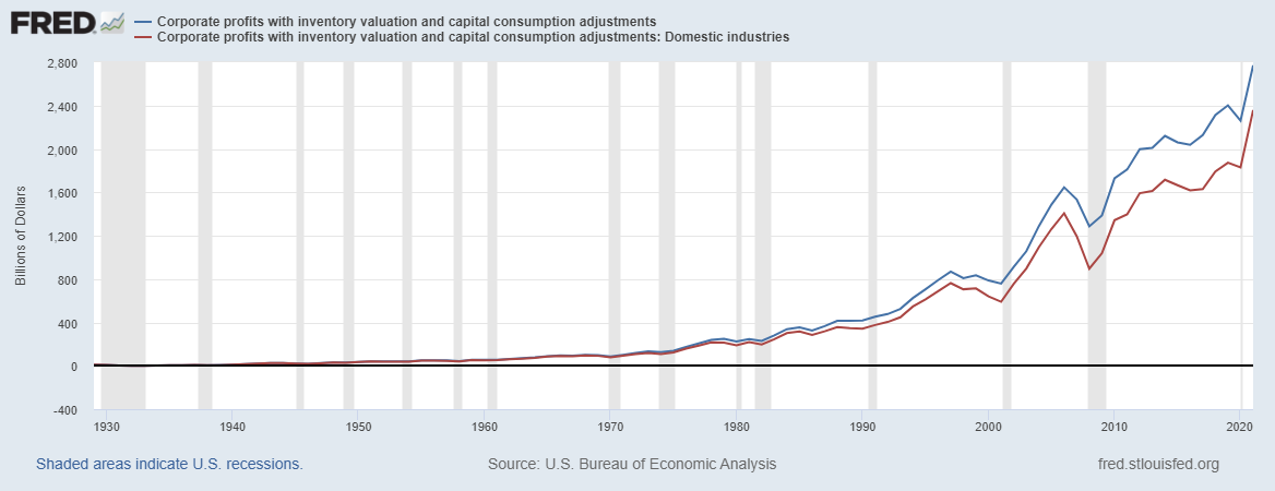
Unlike with employee compensation, national versus domestic does matter a great deal when it comes to measures of profit. Because national profits are profits going to all US residents regardless of where they are located, thus including profits from some production outside the US, they will generally be larger than domestic profits, which are profits from production occurring within the US. This can be seen by comparing the two measures of corporate profits.
Because of this difference in the source of profits, I do not think it is very appropriate to use national income in their comparison with unemployment rates to see evidence for strategic sabotage. Unemployment data is the result of surveys looking specifically at US worksites, and is therefore going to be generally associated with “domestic” rather than “national” production.
As the BLS explains:
“The Current Employment Statistics Program is a federal-state cooperative program. The CES survey is based on approximately 131,000 businesses and government agencies representing approximately 670,000 individual worksites throughout the United States.”
Importantly, my reproduction of their strategic sabotage data was done exclusively in domestic income categories. However, according to Bichler & Nitzan, they went ahead and redid their examples using domestic categories and got the same results as they did originally, showing a clear parabolic relationship with profits and unemployment. Compare this to my replication, which showed a tenuous statistical relationship. What then is the cause of this difference?
The answer lies in the difference between gross and net domestic product. The BEA defines net domestic product as follows:
“The market value of the goods and services produced by labor and property in the United States less the value of the fixed capital used up in production; equal to gross domestic product (GDP) less consumption of fixed capital (CFC). NDP may be viewed as an estimate of sustainable product, which is a rough measure of the level of consumption that can be maintained while leaving capital assets intact.”
The key difference between the two is that net does not include the consumption of fixed capital while gross does. All of Bichler & Nitzan’s graphs, including their new updated ones in response to me, use Net rather than Gross, therefore excluding the consumption of fixed capital aka depreciation, from their analysis. They insinuate that I made a mistake by looking at gross income rather than net, but the truth is that I was being generous, steel-manning their argument as best as I could. Excluding the consumption of fixed capital means that they are not producing any unique results compared to the neoclassical or marxist economists they originally set out to critique.
To elaborate, let me bring back a point I made earlier about the Kalecki-Profit equations. Kalecki is forced to include depreciation as a part of profit because depreciation corresponds to a part of income, the revenue that firms and individuals receive, but it doesn’t correspond to any actual cost they are taking on, like wages are. Had Bichler & Nitzan wanted to eliminate the category of depreciation while still accounting for all income, they should have added it to profits. Depreciation occurs because we have to at some point account for the costs of the means of production, which are purchased as investments. The custom is to account for them as they are used up, and this creates the depreciation schedule which is based on an estimate over how long the fixed capital will last. The schedule is adjusted if the fixed capital lasts shorter or longer than the depreciation schedule would suggest.
As the BEA suggests, depreciation is earmarked as a part of income so that the existing capital stock can be reproduced and maintained, the point of excluding it is to focus on what part of income can be directly consumed. For firms, even though they control this revenue in the present, and could, per the Kalecki equations, theoretically move the cash towards consumption by the capitalist class, they must still account for the original investment in the books. Fixed investment, by its very nature of using real economic resources, does mean less consumption when the means of production are being produced. By representing the costs of the means of production in this way, depreciation exists as a social method for ensuring that the means of production are continually reproduced using the revenue of today, the more depreciation that a firm has, the less of its revenue can be practically sent to the capitalists for consumption.
By ignoring depreciation and fixed capital consumption, the CasP theorists ensure that the primary mover of changes in profit are changes in wages, enforcing their hypothesis that capitalists will sabotage production in order to drive down wages. Their focus on capital as a financial source of power which is struggling for income against labor conveniently leaves out the other major determination of income to capitalists, which is the costs of the means of production. CasP theory cannot accept this fact because it is counter to their central foundations that rejects the importance of the technical aspects of production in determining income, that the nominal is not a reflection of the real economy.
I have done plenty of research that suggests that strategic sabotage does exist (see my previous articles: 1 2 3 4 ), but it certainly doesn’t exist by simply slowing down production. Besides explicit state policies that favor capital over labor, the primary method of strategic sabotage in neoliberalism has been the failure of capitalists to invest in fixed capital.
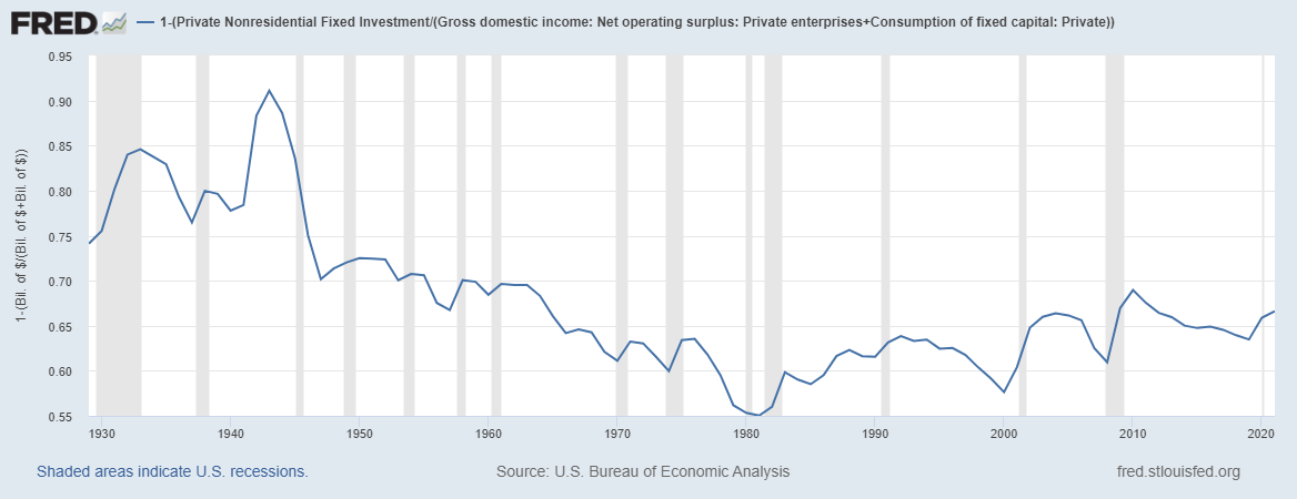
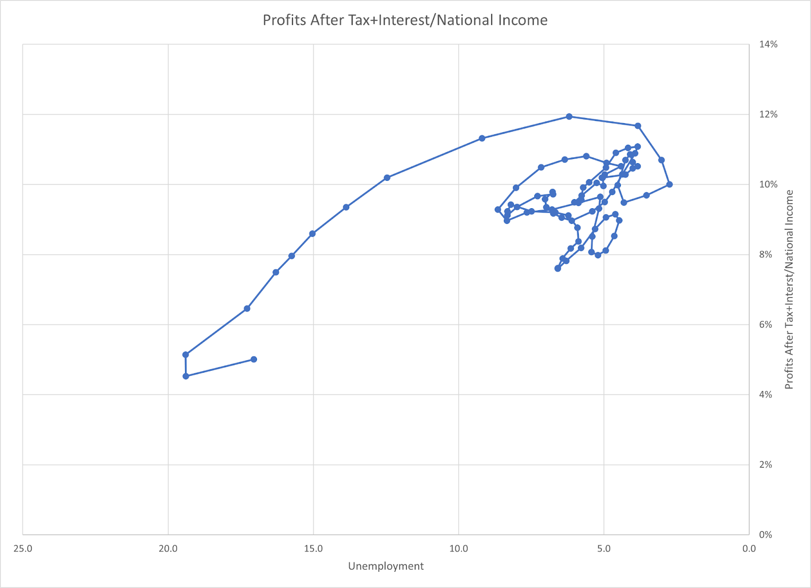
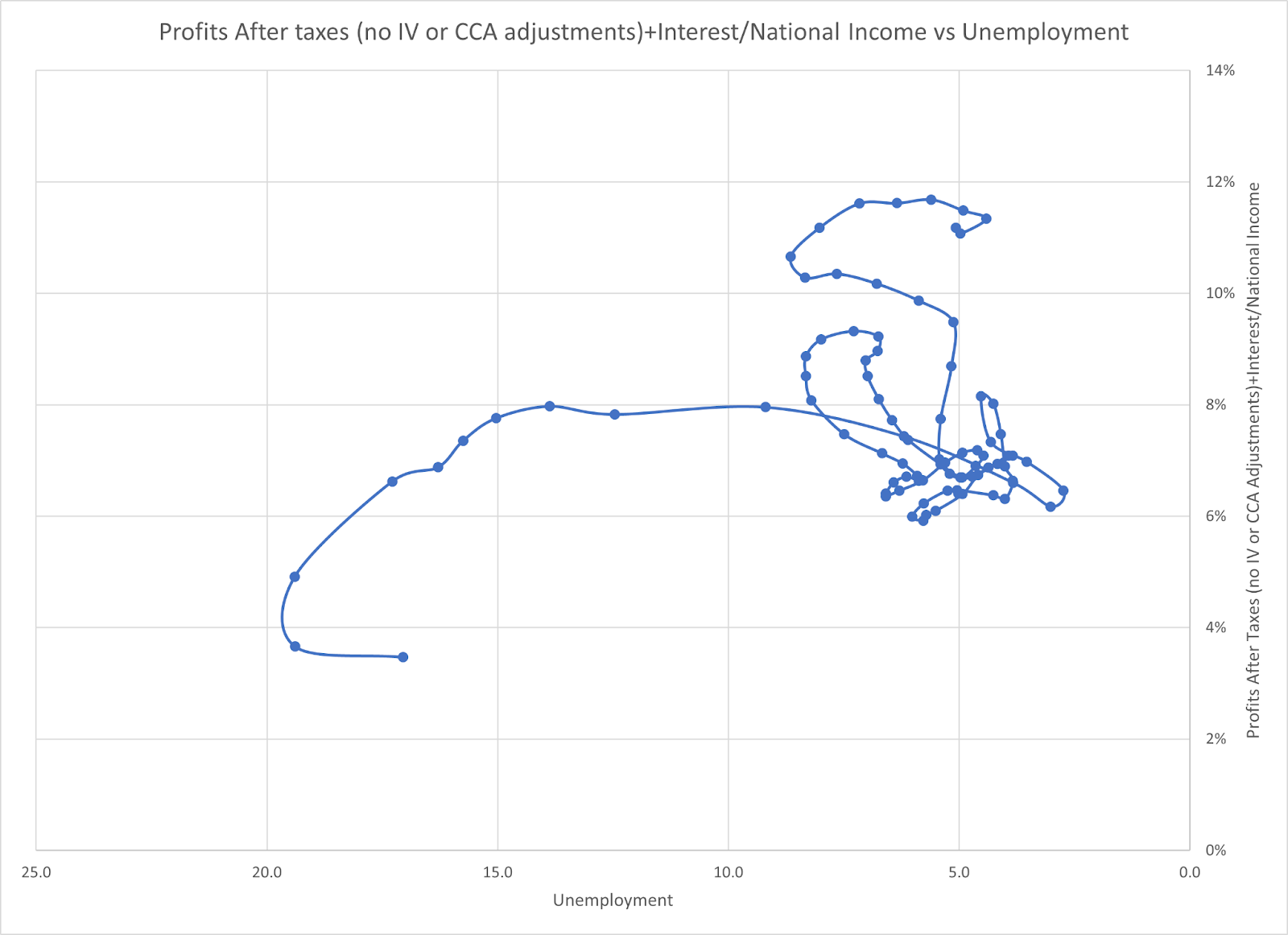
When you include consumption of fixed capital by using gross domestic data, you get the results that I did in my previous post, which doesn’t reveal any particular parabolic relationship between profit and unemployment.

.
.
.
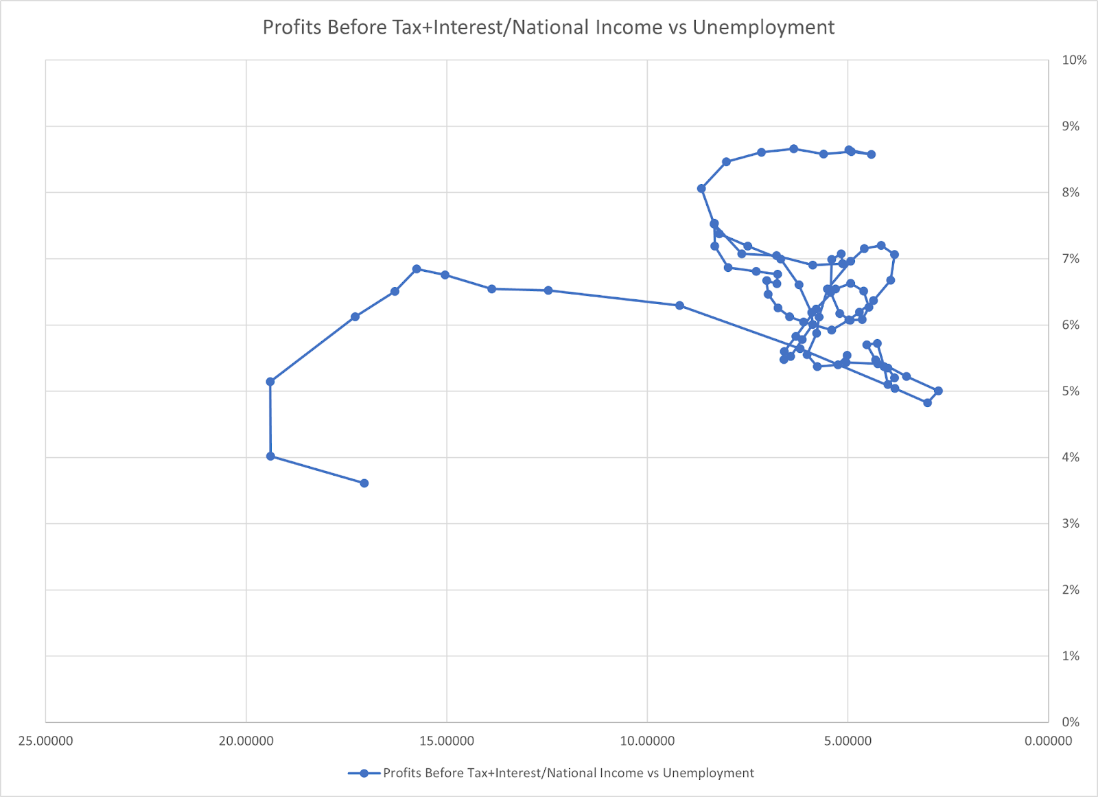
Source: profit/national income.
Why is real production and depreciation so important to capitalists? It’s because when profit, in the Kaleckian sense, is controlled by the technical requirements of production through the demand of reproducing the means of production, capitalists can no longer control or consume it. When you leave out depreciation, you are essentially left with the marxist concept of the rate of exploitation, which, as we have illustrated previously, also has a very large impact on profits. But, crucially, the idea that the split of income between workers and capitalists would be tilted to workers in periods of very low unemployment is something that both neoclassical economists and marxists can easily accept, it is not a new, revolutionary notion in political economy, nor does it explain what determines profit in general.
The rejection of depreciation and investment as key factors in determining profit necessarily consigns CasP theory to an unscientific and idealist status. In order to understand contemporary politics and economics, an understanding of capital and labor in their material forms, in the creation of machinery, in the length of the working day, is absolutely essential. If CasP theorists would like to make their theory more than an assemblage of trivial economic facts and political science indexes, they would do well to try to understand the reality of the capital stock and depreciation as they apply to firms and the capitalist class.
Why would you even bother replying to those capital as power guys? Their entire argument relies on false statements (like industry and bussiness being seperate and orthogonal, something imperically false as shown by things like planned obsolecense, a tendency that is present in all industries) and complete horsecock like "profits come from 'sabotage' " whatever the fuck sabotage means, after which they claim unemployment is equal to sabotage and try to prove their asspull "good amount of sabotage" curve by using data that looks like a bouquet of flowers.
Fucking Austrian economics is more coherent than whatever that was.