
The Social Architecture Model, now with fixed capital
My research in agent based models and classical econophysics

I’ve been vocal that I believe that the field of classical econophysics, which has its roots in the works of Marxist economists bringing statistical mechanics into economics, is on the true cutting edge of economics today. Unlike the emphasis of neoclassical economics, with its insistence on its foundation in the subjective calculus of demand functions, this new field allows for an agnosticism about the desires of subjects. It accomplishes this, essentially, by looking at what happens when we apply simple rules to these agents that engage in random transactions with one another, imposing a social architecture on them.
One of the major advances in classical econophysics was the creation of the social architecture model as formulated by Ian Wright. This model, first introduced in 2004, took what had been the basics of econophysics up to that point, randomly exchanging agents, and added a labor market and firms, whereby agents would be hired by firms and add value to their firms by taking a random slice of the demand on the market and be paid a fixed wage determined by labor market. Since then, there’s been reproductions and modifications by other authors along with Ian, which are summarized here, including one version which provides evidence for the spontaneous creation of Marx’s law of value given very simple assumptions about the relationship of firms and employees.
My humble contribution to this field is to add fixed capital to the model, which up till now has only included wages and labor, as well as make some modest improvements to more closely align with empirical observations. In the future, I’d like to expand the model to include debt, as well as different production departments as Marx did in capital volume 2.
The Social Architecture model has previously been able to replicate distributions of populations in social classes, which are generally normal distributions, as well as income distributions which capture a gamma distribution for working class income and a pareto distribution for capitalist class income, the distribution of firm deaths as well as profit rates compared to those found empirically. One of the biggest problems for the social architecture model has been its results which produce unusually high levels of unemployment, with averages around 12% or greater for example. My model solves this problem, however, there are some lingering issues with a tradeoff in producing a more accurate income distribution vs more accurate unemployment and wage shares of income.
The code for my model can be found here, it’s run in R.
Setup
Each agent has the following attributes:
ID: A Unique ID to differentiate it from other agents
Money: Amount of money agent currently has, each agent begins with 100
Employment Index: This is for worker agents, it contains the ID of their employer
Wage Level: If an agent is employed this contains their current wage rate.
Wage Expectation: The minimum expectation for an agent to accept a wage offer if they went into the job market.
Constant Capital: This is for employer agents, it’s the amount of constant capital owned by their business.
Variable Capital: This is for employer agents, it’s the amount of wages they’ve paid for a given production cycle.
Revenue: The amount of money an agent receives in a given production period.
Number of Employees: Number of people currently employed by an employer agent.
Exogenous variables include the depreciation rate, the limit of the fixed capital investment to wages ratio, and the savings rate for capitalists. As a default, depreciation is set to 15%, the fixed capital investment ratio limit is set to 40%, and the savings rate set to 50%.
Step One: Depreciation
If there is constant capital in employer accounts, it is depreciated by the exogenous depreciation rate for this production cycle.
Step Two: Turn Order Determined
A randomized list of agents is produced to decide the order of “turns”, each agent goes once per production cycle.
Step Three: Hiring process
Agents that are not employers (workers and the unemployed) enter the labor market. A list of potential employers is created from the list of employers and unemployed that excludes the current agent, and which excludes those agents that have no money. A potential employer is randomly chosen, weighted by their wealth. The wealth weighting is accomplished by dividing a potential employer’s wealth by the sum of all the potential employer wealth.
The wage offer is set to the agent’s wage expectation.
If the potential employer has more money than wage offer, plus the limit of capital to worker costs for the offer, and the wage offer is greater than the current wage level for the agent, the offer is accepted. When the offer is accepted, wage expectations increase by 2%. If the offer is rejected and the agent is unemployed, wage expectations go down by 40%.
Step Four: Consumption
One of the other agents which has positive money is randomly chosen from a uniform distribution to consume. The cost of the consumption is a random amount between 1 and the total amount of money held by this other agent. This amount is added to the latent demand, and subtracted from this other agent’s money account.
Step Five: Worker’s Add Value to Firm
If the agent is a worker, they will sample the latent demand to add value to the firm with their labor. The value added will be a random (uniform distribution) amount between 1 and the total latent demand. The amount sampled from the latent demand will be subtracted from the latent demand and added to the employer’s money account.
Step Six: Employer Value Add
The same sampling process repeats itself, except value is added to the agent’s own account.
Step Seven: Wage Payment
A random capital expense ratio is chosen between .1 and the exogenous limit.
An array with three rows is created, the first row is for the IDs of worker agents, the second row is for their wage levels, and the third row is for their wage level plus the capital expenses associated with those wage expenses. The columns of this array are then randomized. An amount of wage and capital expense bundles are chosen whose cumulative sum is less than the amount of money the employer has, these expenses are paid. Agents whose wages cannot be paid are laid off. The wages are added to the worker’s money accounts and subtracted from the employer’s. The capital expenses are added to the latent demand and subtracted from the employer’s money account and moved onto their books as constant capital.
Step Eight: Bankruptcy
If an employer no longer has any employees it enters bankruptcy. The firm’s constant capital is transferred to another randomly chosen, via a uniform distribution, employer. The constant capital, variable capital, and revenue accounts for the employer are zeroed out.
At any given time interval, the relevant processes are undertaken per agent, and the whole process repeats for the amount set at the beginning, the standard being 12000 times. Included in my code are graphs which will be automatically produced when run in R that document the outputs.
Results
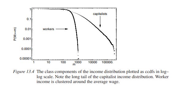
In terms of income, I was able to replicate the pareto distribution for the upper end of the income distribution and a gamma distributed lower end.
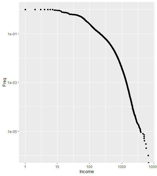
The black dots are the model output points and the orange line is a randomly generated and normalized pareto distribution with a scale of 1e3 and shape of 5.3. For some reason, I found it easier to generate a large of number of points in a pareto distribution rather than making a pareto curve directly in R for a cumulative graph like this.
Unfortunately, the difference between capitalist and worker income is not quite as distinct as it is in previous experiments.
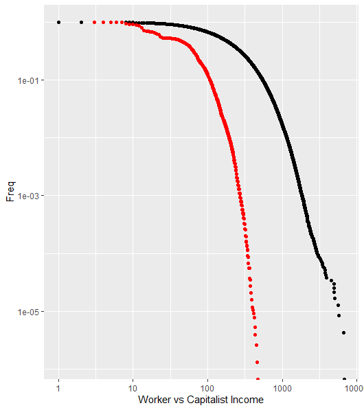
Compare this to data from the SA model discussed in the book Classical Econophysics.
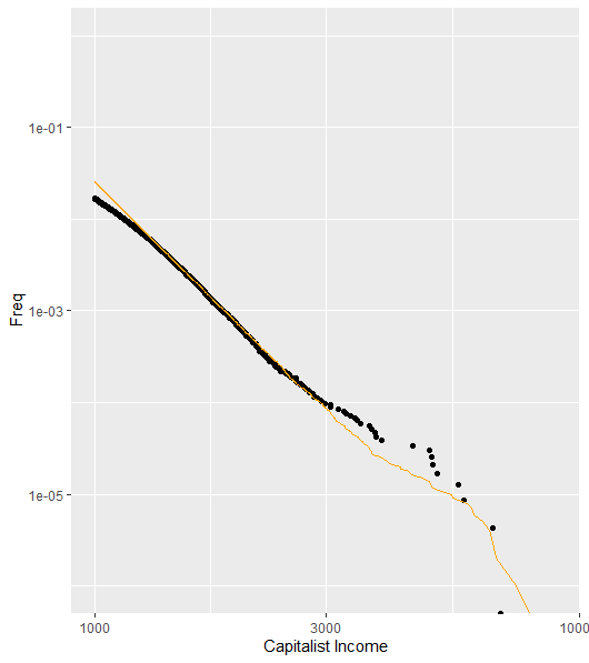
We can zoom in on the non-cumulative distributions to more clearly see the gamma and pareto distributions.
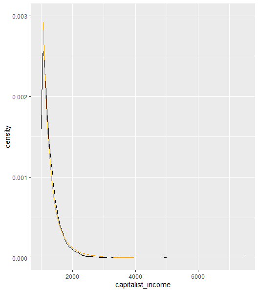
Here’s the capitalist income with a pareto distribution of a scale of 1000 and a shape of 4.
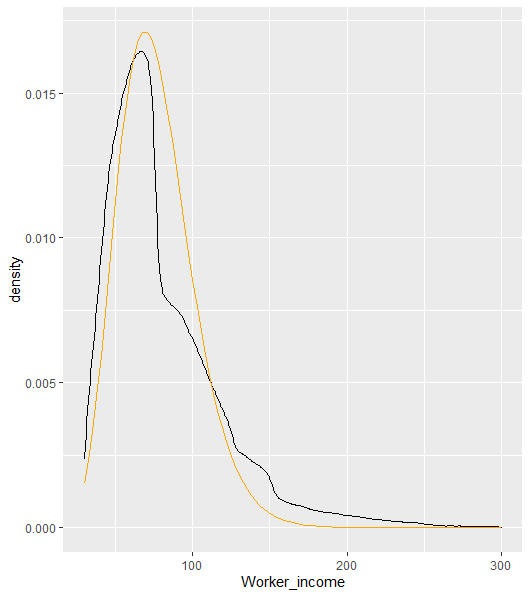
Here’s the worker income distribution compared to a gamma distribution with a shape of .13 and a scale of 10.
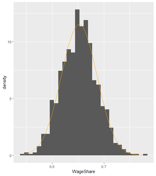
One thing my modified social architecture model was able to approximate very well was the wage share of income, with an average of 65%, compared to a real life average of 62% in the US, and 65% in Germany.
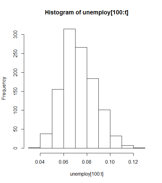
Unemployment
One big change in my model compared to previously are the harsh penalties for not finding a job in the labor market, namely a 40% decline in wage expectations for unemployed failed job seekers, and only a 2% gain from finding a job or changing positions. While this has produced outcomes far more in line with quantitative observations of real economies, it is not without its problems as an assumption. One generous interpretation is that this severe decline in wage expectations is analogous to an individual pessimistic about their prospects simply taking whatever work they can.
Unlike previous models which have had average unemployment levels at 12% or greater, this approach has yielded unemployment rates at around an average of 7%, which can be compared to 5.7% in the US and 6.8% in Germany for the data we have on record.
Fixed Capital
What is totally new in this model, however, is the addition of fixed capital. In this model, all fixed capital does is exist as a cost and accumulate over time. In some versions I experimented with, I also included a bonus for a firm having fixed capital where the capital intensity would give it a greater fixed share of latent demand, or a competitive advantage relative to other firms, however these changes had no effect on the macro level outputs, which is why I left it out in the final version. Unlike variable capital, payments for fixed capital are treated like the consumption expenditures on goods, going towards latent demand rather than wage payments to workers. In my initial attempts, I had these decisions to invest made the same way as consumption decisions by capitalists, with random expenditures from their cash reserves, but this caused the rate of profit to positively correlate with capital intensity which is the opposite of empirical observations. The best outcome came from determining investment decisions with a technical ratio opposite wage rates, such that when wage payments were made a random amount between 10-40% was also invested in fixed capital.
When firms go bankrupt, another random firm received their fixed capital at no charge; fixed capital was only destroyed by regular depreciation. This is somewhat analogous to how firesale assets are passed on, but more importantly, I believe that in order to calculate the full cost of fixed capital it would be necessary to add on specific financial capital markets.
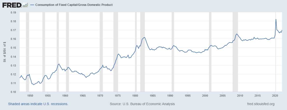
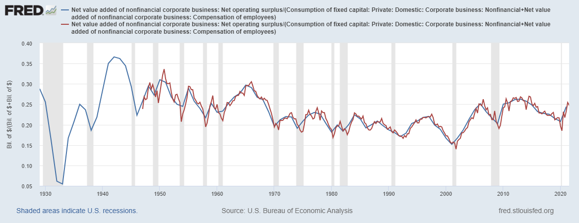
Regardless, the accumulation of capital resulting from the model was strikingly similar to what we have in empirical data.
As you can see, constant capital depreciated as a share of revenue continued to grow for about 50-60 years until investment reached an equilibrium with depreciation.
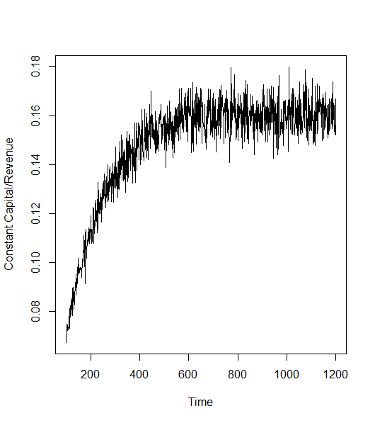
The equilibrium it reached was at roughly 15-17% depreciation as a share of revenue, which matches up with the empirical data in the US.
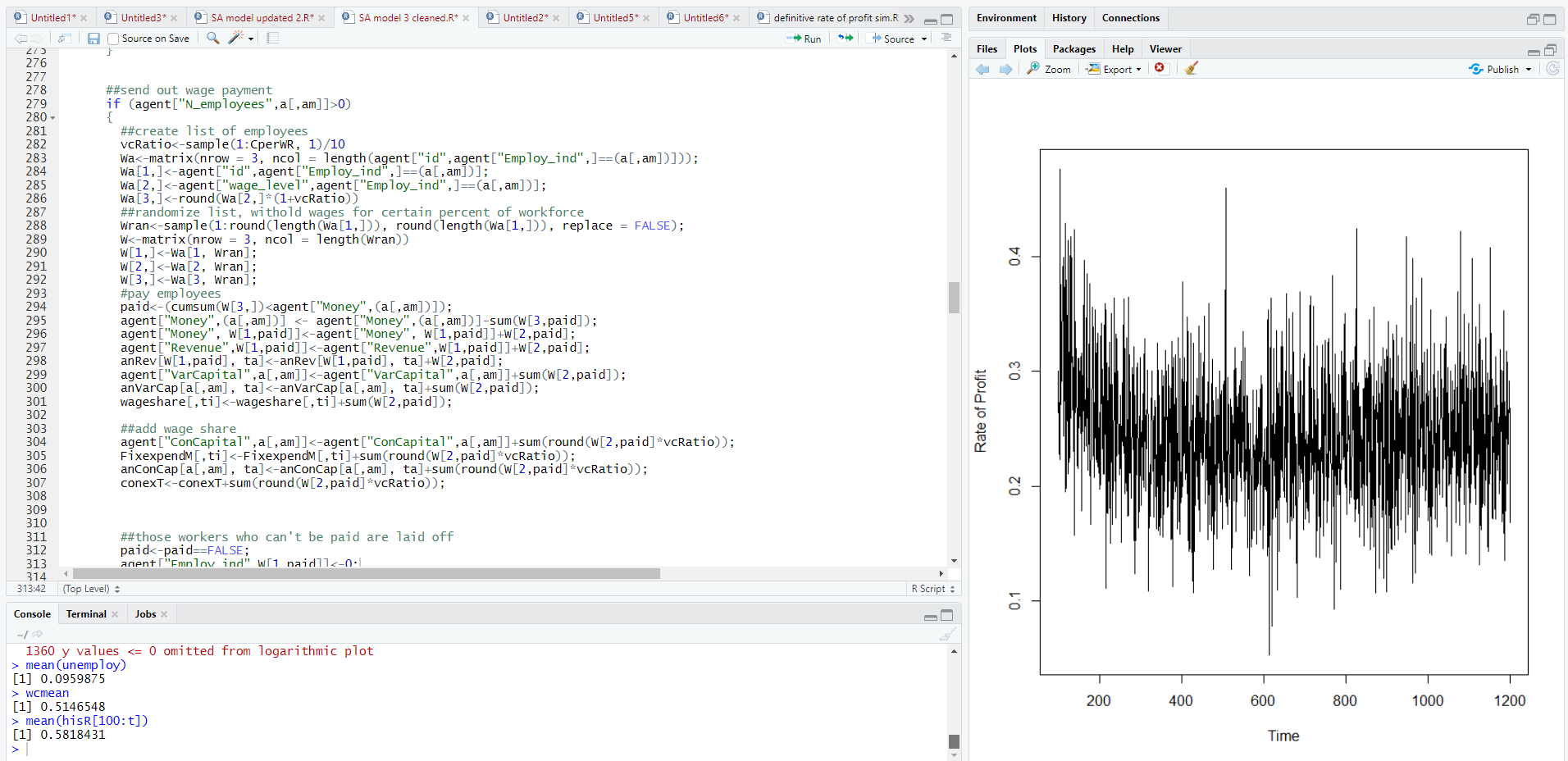
Rate of Profit
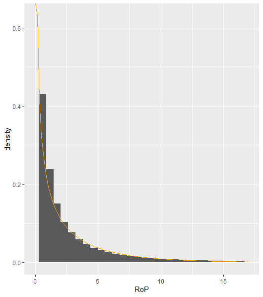
The average rate of profit in the simulation was 24%, not too far off from the US nonfinancial rate of profit average of 23%.
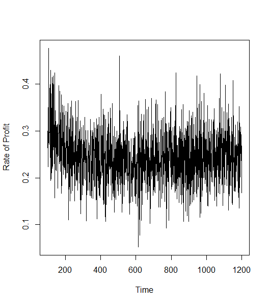
In terms of the distribution of that rate of profit among firms, it matches with other empirical and simulation data which finds a gamma distribution of profit rates. In this case the orange line gamma distribution has a scale of .15 and shape of .4.
As was mentioned earlier, since this model includes fixed capital it’s important that it reflect the key insight of classical econophysics that profit rates and capital intensity be negatively correlated. This is confirmed by the following plot and regression.
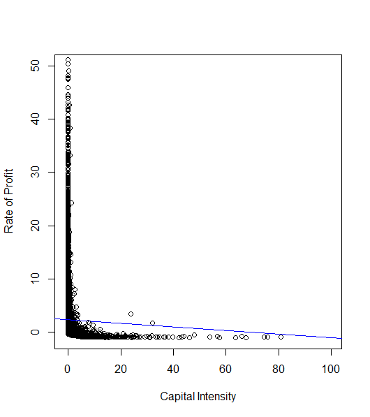
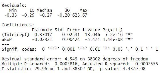
Unfortunately, it’s not a very pretty plot, mostly due to the low level of aggregation. In most of the studies that confirm the correlation, they’re on the level of industry aggregates.
Capitalist Consumption Limit aka Capitalist Savings
One of the exogenous variables listed was capitalist savings, in this case, the variable controls the limit capitalists can consume for themselves at any given moment, which is otherwise a random amount of money from the amount they currently have in their account. In reality, capitalists have strong incentives not to consume all of their money, as they live off the income which is a return to their capital, that is wages and fixed capital money advances for production. The less money they consume, the more they can spend on wages and investment. In the social architecture model, there is no distinction between firm accounts and capitalist individual accounts - in reality capitalists would likely be unable to fully liquidate all of the cash reserves they technically own, as firms must approve the disbursement of dividends, thus there is reason to believe this limit in real economies is non-zero and possibly quite significant.
Changing the level of capitalist savings from 50% to 0% produces some significant differences, including higher rates of unemployment (10%), lower wage share (51%), lower constant capital as a share of revenue (11-13%), and much higher rates of profit (60%). Evidence that supports my conjecture that preserving capitalist consumption is a major fetter on the economy, which you can read more about here, here and here.
One metric which capitalist consumption does increase is firm revenue, highlighting the important difference between real and nominal GDP which was discussed in this overview of the social architecture model. Nominal GDP can essentially be treated as revenue to firms, but in terms of real output, we can assume it’s a result real activity, that is work by those employed in a given period. Even without introducing changes in the amount of money in the system, real and nominal GDP can diverge in the method outlined here, via changes to capitalist consumption behavior.
The below are a comparison of various metrics of various metrics in the 50% and 0% capitalist savings simulations, pay attention to the scales.
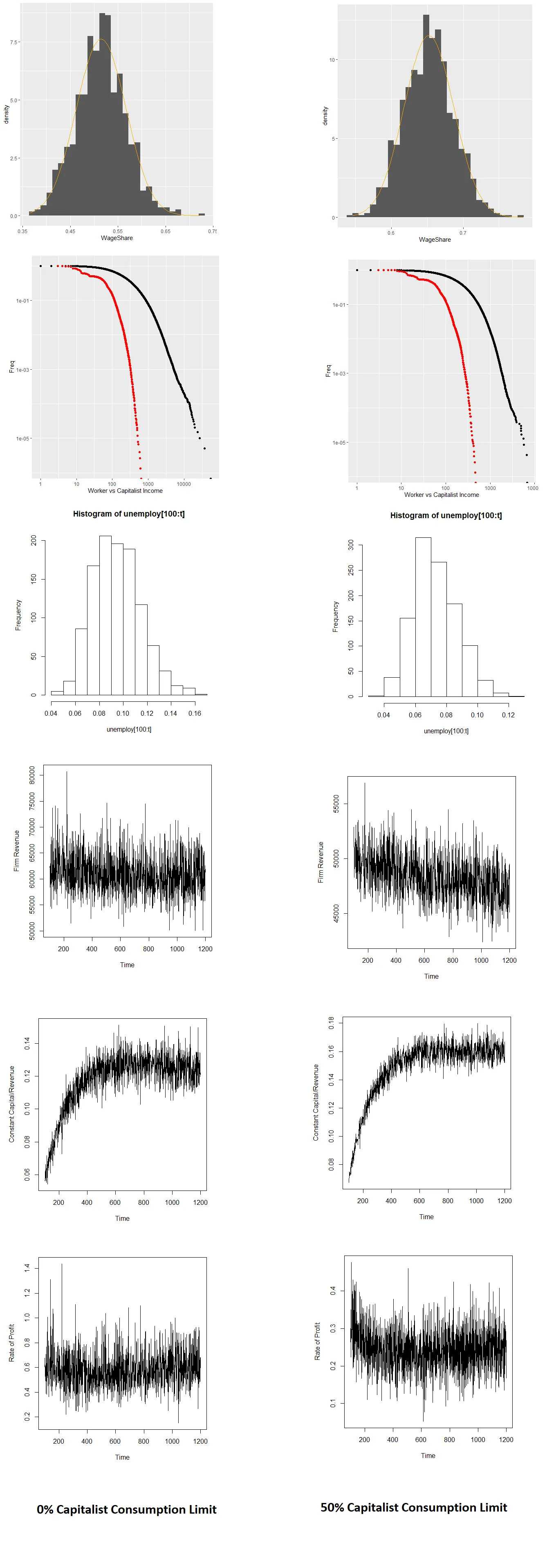
This difference resulting from capitalist consumption behavior is a concrete prediction of the model, and one that might be worth investigating in the future.
Hopefully I will be able to devote more time to econophysics and agent based modeling in the future, as it is one of my favorite obsessions. If you’d like to support my work be sure to sign up for a subscription.